Disease Progression Models
1 Stable vs. Progressive Disease
ME/CFS trajectories vary substantially: some patients remain at a stable severity level for years, others progressively worsen, and a minority improve spontaneously (Brurberg et al. 2014). The integrated model explains these trajectories through the balance between damage accumulation and repair:
\[ \frac{d D_\text{total}}{d t} = k_\text{damage} \cdot [\text{ROS}] + k_\text{immune}_{\text{damage}} \cdot \mathbf{C}_\text{pro} - k_\text{repair} \cdot \frac{[\text{ATP}]}{K_\text{repair} + [\text{ATP}]} \tag{1}\]
where \(D_\text{total}\) is aggregate tissue damage (encompassing mitochondrial damage, neuronal injury, endothelial dysfunction), \(k_\text{damage}\) and \(k_\text{immune}_{\text{damage}}\) are damage rates from oxidative stress and inflammation respectively, and \(k_\text{repair}\) is the ATP-dependent repair rate. Three regimes emerge:
- Stable disease: damage and repair rates are balanced (\(d D_\text{total} \\/ d t \approx 0\)). The patient remains at a constant severity level determined by the equilibrium damage.
- Progressive worsening: damage exceeds repair (\(d D_\text{total} \\/ d t > 0\)), often because the energy deficit limits repair capacity. The resulting damage further impairs energy production, creating a slow positive feedback loop that produces gradual decline over months to years.
- Gradual improvement: repair exceeds damage (\(d D_\text{total} \\/ d t < 0\)), possible when successful pacing or treatment reduces ROS and inflammation sufficiently for repair processes to dominate. This predicts that sustained activity management is a prerequisite for recovery, consistent with the energy envelope theory (Jason et al. 2012).
2 Relapse–Remission Patterns
Many ME/CFS patients experience cyclical symptom patterns with periods of relative improvement followed by relapse. The integrated model can produce such patterns through two mechanisms.
Exogenous cycling: External perturbations (infections, physical overexertion, hormonal cycles) periodically push the system away from its steady state, producing transient symptom flares followed by partial recovery. The severity and duration of each relapse depend on the perturbation magnitude and the system’s recovery capacity. Repeated perturbations before full recovery produce a “staircase” pattern of progressive worsening—each cycle reaches a lower functional nadir than the previous one.
Endogenous oscillations: As noted in Chapter Integrated Multi-System Models, the feedback structure of the coupled system may produce limit cycle oscillations without external perturbation. If the ME/CFS parameter regime places the system near a Hopf bifurcation, small noise can excite large-amplitude oscillations with irregular periodicity, producing the apparently random symptom fluctuations reported by patients.
3 The Energy Ratchet: A Discrete Event Model
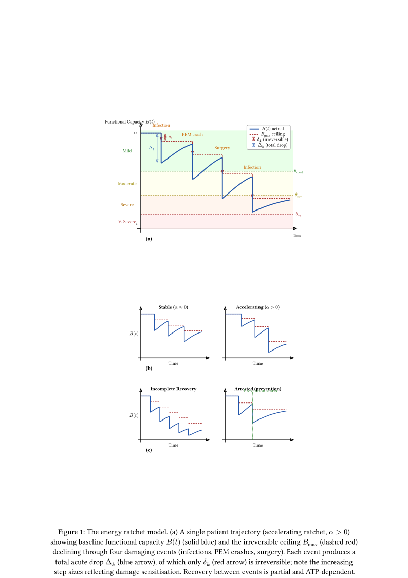
The continuous damage model (Equation damage accumulation) captures gradual progression but does not represent the discrete, step-wise decline observed in ME/CFS. While infections are a major trigger (Speculation~Infection-Induced Irreversible Damage: The Ratchet Model), the ratchet pattern extends to any event that forces energy expenditure beyond the recoverable envelope: PEM-inducing overexertion, surgical stress, emotional trauma, or hormonal shifts. We therefore formalise a general energy ratchet as a hybrid dynamical system combining continuous inter-event repair dynamics with discrete event-triggered damage jumps.
3.1 State Variables and Inter-Event Dynamics
Let \(B(t) \in [0,1]\) denote baseline functional capacity (1 = healthy, 0 = complete disability) and let damaging events (infections, PEM crashes, surgeries, major stressors) arrive at discrete times \(t_1 < t_2 < dots.c\). Between events, the system evolves under continuous repair:
\[ \frac{d B}{d t} = r(B) \cdot \frac{[\text{ATP}]}{K_\text{repair} + [\text{ATP}]} \cdot (B_max (t) - B(t)), \quad t \in (t_k, t_{k+1}) \tag{2}\]
where \(r(B)\) is a repair rate that decreases with accumulated damage (reflecting reduced regenerative capacity), \([\text{ATP}] \\/ (K_\text{repair} + [\text{ATP}])\) is the energy-dependent repair term from Equation damage accumulation, and \(B_max (t)\) is the current ceiling—the maximum baseline the system can recover to, which is itself modified by each damaging event (see below). The key asymmetry is that \(B\) relaxes toward \(B_max\), but \(B_max\) can only decrease.
3.2 Damaging Events: The Ratchet Jump Map
At each event time \(t_k\), two discrete updates occur:
\[ \begin{aligned} B_max (t_k^+) &= B_max (t_k^-) - \delta_k \\ B(t_k^+) &= B(t_k^-) - \Delta_k \end{aligned} \tag{3}\]
where \(\delta_k > 0\) is the irreversible ceiling loss—the permanent downward ratchet step—and \(\Delta_k > \delta_k\) is the total acute functional drop (which includes the reversible component that can be partially recovered between events). Both values are clamped so that \(B\) and \(B_max\) remain in \([0,1]\). The irreversible fraction depends on event severity \(S_k\), event duration \(\tau_k\), and the patient’s current damage state:
\[ \delta_k = \delta_0 \cdot S_k \cdot (1 + \alpha \sum_{j<k} \delta_j) \cdot (1 - e^{-\tau_k \\/ \tau_\text{crit}}) \tag{4}\]
Here \(\delta_0\) is a baseline vulnerability parameter (patient-specific), \(\alpha \geq 0\) controls damage sensitisation (prior damage amplifies future damage, producing accelerating decline), and \(\tau_\text{crit}\) is a critical event duration beyond which damage saturates. In the general model, \(\delta_0\) and \(\tau_\text{crit}\) may differ by event type (e.g., \(\delta_0^\text{inf}\) for infections, \(\delta_0^\text{PEM}\) for overexertion); for parsimony, we present the single-parameter form here. The term \((1 + \alpha \sum_{j<k} \delta_j)\) formalises the positive feedback loop identified in the qualitative model: for infections, this captures microglial priming and immune exhaustion; for overexertion events, it captures progressive mitochondrial damage and reduced metabolic reserve. In both cases, each event leaves the system more vulnerable to the next.
3.3 Recovery Dynamics and Asymmetry
Between events, Equation ratchet interevent drives \(B(t) -> B_max\) exponentially with effective time constant:
\[ \tau_\text{rec} (B) = \frac{1}{r(B)} \cdot \frac{K_\text{repair} + [\text{ATP}]}{[\text{ATP}]} \tag{5}\]
The ratchet asymmetry emerges because \(\tau_\text{rec}\) increases as \(B\) decreases—sicker patients recover more slowly (reduced ATP availability impairs repair). If the inter-event interval \(t_{k+1} - t_k < 3 \tau_\text{rec}\), the patient has not recovered to within approximately 5% of \(B_max\) before the next hit (exact fraction depends on how \(r(B)\) and \([\text{ATP}]\) vary during recovery; the 5% estimate assumes roughly constant effective rate), producing the “staircase” pattern described in Section Disease Progression Models. In this regime, the effective baseline drops faster than the ceiling alone would predict, because each event strikes before recovery is complete. This applies equally to closely-spaced PEM crashes (e.g., a patient repeatedly exceeding their energy envelope) and to recurrent infections.
3.4 Severity Transitions and Critical Thresholds
Clinical severity levels correspond to threshold values of \(B\):
\[ \begin{aligned} \text{Severity}(t) = cases( \text{mild} & B(t) > \theta_\text{mod}, \text{moderate} & \theta_\text{sev} < B(t) \leq \theta_\text{mod}, \text{severe} & \theta_\text{vs} < B(t) \leq \theta_\text{sev}, \text{very severe} & B(t) \leq \theta_\text{vs} ) \end{aligned} \tag{6}\]
with approximate thresholds \(\theta_\text{mod} \approx 0.6\), \(\theta_\text{sev} \approx 0.35\), \(\theta_\text{vs} \approx 0.15\) (to be calibrated against functional capacity scores).
3.4.1 Extended Severity Classification for the Extremely Severe Range
The standard four-level classification (Equation ratchet severity) collapses all patients below \(\theta_\text{vs}\) into a single category. Jahanbani et al. proposed a finer-grained scale that subdivides the very severe range into five extremely severe sub-levels (A through E, with E the most profound) (Jahanbani et al. 2024). This reflects clinical observations that patients at the bottom of the severity spectrum exhibit meaningful differences in functional capacity—ability to communicate, tolerate sensory input, or take nutrition orally—that the coarse classification obscures. The model accommodates this refinement by partitioning the very severe range into equal-width bands:
\[ \begin{aligned} \text{Sub-level}(t) = cases( \text{VS} & \theta_\text{es} < B(t) \leq \theta_\text{vs}, \text{ES-A} & \theta_\text{es} - w < B(t) \leq \theta_\text{es}, \text{ES-B} & \theta_\text{es} - 2w < B(t) \leq \theta_\text{es} - w, \text{ES-C} & \theta_\text{es} - 3w < B(t) \leq \theta_\text{es} - 2w, \text{ES-D} & \theta_\text{es} - 4w < B(t) \leq \theta_\text{es} - 3w, \text{ES-E} & B(t) \leq \theta_\text{es} - 4w ) \end{aligned} \tag{7}\]
with \(\theta_\text{es} \approx 0.10\) and band width \(w = \theta_\text{es} \\/ 5 = 0.02\) (thresholds to be calibrated against the Jahanbani functional descriptors). The equal-width partition is deliberate: it is not the thresholds that need a nonlinear transformation, because the dynamics already supply the compression.
3.4.2 Biophysically Grounded Recovery Asymmetry
The recovery time constant (Equation ratchet recovery time) depends on both the repair rate \(r(B)\) and the energy-dependent repair term:
\[ \tau_\text{rec} (B) = \frac{1}{r(B)} \cdot \frac{K_\text{repair} + [\text{ATP}](B)}{[\text{ATP}](B)} \]
Rather than assuming linear proportionalities (\([\text{ATP}] \propto B\), \(r \propto B\)), both relationships can be derived from the biophysics already in the model (Chapter Energy Metabolism Models).
3.4.2.1 ATP: Three Regimes from the ATP Synthase Threshold
The ATP synthase equation (Equation atp synthase) gives ATP production as a function of the mitochondrial membrane potential \(\Delta \Psi\):
\[ J_\text{ATP synthase} \propto \frac{\Delta \Psi - \Delta \Psi_\text{threshold}}{\Delta \Psi} \]
where \(\Delta \Psi_\text{threshold} \approx 110\) mV. Since \(\Delta \Psi\) depends on ETC complex activity (which maps to \(B\) through \(\alpha_\text{CI}\)), steady-state ATP is a piecewise function of \(B\) with three regimes:
\[ \begin{aligned} [\text{ATP}](B) \approx cases( [\text{ATP}]_max \quad & B > B_\text{cliff} \quad & \text{(plateau: } \Delta \Psi \text{>>} \Delta \Psi_\text{threshold} \text{)}, [\text{ATP}]_max \cdot \varphi(B) \quad & B_\text{floor} < B \leq B_\text{cliff} \quad & \text{(cliff: steep } \Delta \Psi \text{drop)}, [\text{ATP}]_min \quad & B \leq B_\text{floor} \quad & \text{(floor: cell-survival minimum)} ) \end{aligned} \tag{8}\]
where \(\varphi(B)\) is the strongly nonlinear cliff function derived from the \(\Delta \Psi\) dependence on Complex I capacity. From the worked example in Section ATP Production Models: a 35% Complex I impairment (\(\alpha_\text{CI}: 1.0 -> 0.65\)) produces a 39% ATP synthase flux reduction—disproportionate because \(\Delta \Psi\) approaches \(\Delta \Psi_\text{threshold}\). This disproportionality is the cliff. Below \(B_\text{floor}\), cells maintain \([\text{ATP}]_min\) (estimated at 15–30% of healthy levels from the ischaemia literature) to avoid apoptosis.
The approximate regime boundaries, mapped from the \(\alpha_\text{CI}\) values in the ch50 worked examples to the \(B\) scale:
- \(B_\text{cliff} \approx 0.65\): above this, \(\Delta \Psi\) is well above threshold (\(> 145\) mV), ATP is near-maximal, and small changes in \(B\) produce small ATP changes (quasi-plateau)
- \(B_\text{floor} \approx 0.05\): below this, \(\Delta \Psi\) is at or below threshold, ATP synthase is minimal, and the cell operates on glycolytic ATP with an apoptosis-prevention floor
3.4.2.2 r(B): Biogenesis–Mitophagy Balance
The repair rate \(r(B)\) is not a free parameter but the net output of two ATP-dependent processes already modelled in Chapter Energy Metabolism Models:
Biogenesis (Equation biogenesis): \(J_\text{biogenesis} = v_\text{bio} \cdot \frac{[\text{AMPK}_a]}{K_\text{AMPK} + [\text{AMPK}_a]} \cdot \frac{[\text{NAD}^+]}{K_\text{SIRT1} + [\text{NAD}^+]}\)
This is a product of two Hill functions with opposing energy dependencies: energy deficit activates AMPK (promoting biogenesis) but depletes NAD+ (inhibiting SIRT1). The net result is a non-monotonic hump: biogenesis peaks at intermediate energy deficit and collapses at severe deficit when NAD+ depletion dominates.
Mitophagy (Equation mitophagy): \(J_\text{mitophagy} \propto \frac{[\text{ATP}]}{K_\text{ATP,autophagy} + [\text{ATP}]}\)
Autophagy requires ATP. Below the critical threshold \([\text{ATP}]_\text{crit,autophagy}\), quality control collapses: damaged mitochondria accumulate because the energy for cleanup is precisely what the damaged organelles fail to produce.
The effective repair rate is therefore:
\[ \begin{aligned} r(B) \approx cases( r_max \cdot (1 - B\\/B_\text{cliff}) \quad & B > B_\text{cliff} \quad & \text{(healthy: mild deficit, AMPK rising, NAD} \text{+} \text{ adequate)}, r_max \cdot \psi(B) \quad & B_\text{collapse} < B \leq B_\text{cliff} \quad & \text{(cliff zone: competing AMPK/NAD} \text{+} \text{ signals)}, r_min \quad & B \leq B_\text{collapse} \quad & \text{(collapse: NAD} \text{+} \text{ depleted, mitophagy stalled)} ) \end{aligned} \tag{9}\]
where \(\psi(B)\) captures the biogenesis hump—initially rising as AMPK activates, then falling as NAD+ depletion dominates—and \(B_\text{collapse} \approx 0.10\)–$ 0.15$ is the threshold where Chapter Energy Metabolism Models predicts quality control failure (\(\gamma < 0.7\), \(J_\text{biogenesis} < J_\text{mitophagy,eff}\)).
3.4.2.3 Recovery Scaling by Regime
Substituting the biophysical functions (Equations atp piecewise and repair piecewise) into the recovery time constant:
\[ \tau_\text{rec} (B) = \frac{1}{r(B)} \cdot \frac{K_\text{repair} + [\text{ATP}](B)}{[\text{ATP}](B)} \tag{10}\]
| Regime | \(B\) range | \([\text{ATP}]\) | \(r(B)\) | \(\tau_\text{rec}\) behaviour |
|---|---|---|---|---|
| Plateau | \(> B_\text{cliff} \\approx 0.65\) | \(\\approx [\text{ATP}]_max\) | Moderate (rising) | Slow, roughly constant — recovery timescale set by \(r\) alone |
| Cliff | \(B_\text{collapse} < B \leq B_\text{cliff}\) | Steep drop (\(\varphi\)) | Hump then decline (\(\psi\)) | Rapid increase — small \(B\) drops cause disproportionate \(\tau_\text{rec}\) increase |
| Floor | \(\leq B_\text{collapse} \\approx 0.10\) | \(\\approx [\text{ATP}]_min\) | \(\\approx r_min\) (collapsed) | \(\tau_\text{rec} \\approx \text{const} \\/ r_min\) — very long, set by collapsed repair machinery |
In the cliff regime (\(B \approx 0.15\)–$ 0.65$, encompassing moderate through severe), both \([\text{ATP}]\) and \(r(B)\) decline with \(B\), producing a steep rise in \(\tau_\text{rec}\). The exact exponent depends on the shapes of \(\varphi\) and \(\psi\), which are determined by the ETC threshold nonlinearity and the AMPK/NAD+ competition respectively. The order of magnitude is consistent with the $ 1\/B^2$ estimate from the linear approximation, but the cliff shape makes it locally steeper than $ 1\/B^2$ near the \(\Delta \Psi\) threshold.
In the floor regime (\(B \leq 0.10\), extremely severe), \([\text{ATP}]\) plateaus at \([\text{ATP}]_min\) and \(r(B)\) has collapsed to \(r_min\). Recovery time is high but no longer divergent—instead, \(\tau_\text{rec} \approx K_\text{repair} \\/ (r_min \cdot [\text{ATP}]_min)\), a large constant. This has a clinical consequence: transitions between adjacent extremely severe sub-levels take approximately equal (very long) times, rather than the quadratically expanding times predicted by the linear approximation. The difference is that between ES-D and ES-E, the patient has hit the biophysical floor—the system cannot get worse in terms of per-unit recovery cost, even though it can still get worse in terms of absolute functional capacity.
The practical consequence across the full range: a moderate patient (\(B \approx 0.50\), in the cliff zone) already experiences significantly prolonged recovery compared to a mild patient (\(B \approx 0.70\), near the plateau), because the ATP cliff amplifies every functional drop. By the severe range (\(B \approx 0.25\)), recovery times have risen by at least an order of magnitude. In the extremely severe range (\(B \leq 0.10\)), the floor regime means recovery times are extremely long but approximately uniform per band—consistent with the observation that patients at ES-C, ES-D, and ES-E all show similarly slow (near-imperceptible) improvement (Jahanbani et al. 2024), without ES-E being dramatically worse than ES-C in rate of improvement per se.
The model therefore predicts that transitions between adjacent extremely severe sub-levels are clinically hard to distinguish not because the underlying biology is static, but because the recovery timescale exceeds typical observation windows. This is an emergent property of the biophysics—the ATP synthase threshold equation, the AMPK/NAD+ competition in biogenesis, and the ATP-dependent mitophagy collapse produce the compression without requiring any fitting assumptions.
The recovery scaling (Equation recovery scaling) describes within-person dynamics: how recovery time changes as a single patient’s functional capacity \(B\) evolves over the disease course. It does not predict that sicker patients recover more slowly than milder patients in cross-sectional comparison. Indeed, Moore et al. found no significant difference in post-CPET recovery time across baseline symptom severity levels (\(F = 1.12\), \(p = 0.33\)) (Moore et al. 2023). This null result is consistent with the model: between-person variation in \(\delta_0\), \(\alpha\), \(r(B)\), and \(K_\text{repair}\) may dominate over the within-person \(B\)-dependence, and the CPET protocol itself excludes the most severely affected patients who cannot exercise, truncating the severity range over which the scaling would be most pronounced. Empirical validation requires longitudinal within-person tracking across severity transitions—data that do not yet exist but that home-visit protocols such as ACHTSAM (Fricke et al. 2026) and instruments such as FUNCAP (Sommerfelt et al. 2024) (designed to avoid floor effects at the extreme end) may enable.
The boundaries \(B_\text{cliff} \approx 0.65\) and \(B_\text{collapse} \approx 0.10\) are estimated from the ch50 worked examples (\(\alpha_\text{CI}\) values mapped to \(B\)) and the NAD+ depletion threshold (\(\gamma < 0.7\)). The true boundaries are patient-specific, depending on individual mitochondrial reserve, antioxidant capacity, and NAD+ metabolism. Numerical integration of the full coupled ODE system (Equations atp synthase, biogenesis, mitophagy with patient-specific parameters) would yield precise \(\tau_\text{rec}(B)\) curves; the piecewise description here captures the qualitative regime structure.
The recovery time constant \(\tau_\text{rec}(B)\) (Equation recovery scaling) describes how rapidly \(B(t)\) relaxes toward the current ceiling \(B_\max(t)\) within inter-event dynamics (Equation ratchet interevent). It does not describe escape from the disease attractor itself. The bistability analysis (Chapter Integrated Multi-System Models, Section Hysteresis and the Intervention Window) treats the entire disease state—including all \(B\) values up to \(B_max\)—as a stable basin sustained by positive feedback among energy depletion, immune dysregulation, ROS, and inflammation. Even after a patient has fully relaxed to \(B = B_max\) via slow endogenous repair (potentially years in the floor regime), the system remains within the disease basin. True recovery requires crossing the separatrix into the healthy attractor, which is biophysically distinct from intra-basin relaxation.
Two implications follow.
Pharmacological recovery is parameter modification, not amplification of endogenous repair. Effective treatments work by shifting parameter values (raising \(\alpha_\text{CI}\), lowering \(k_\text{exh}\), modifying \(K_\text{MC}\), and others) until either the disease attractor shrinks enough that noise-driven escape becomes feasible (Section Endogenous Oscillations and Hopf Bifurcation) or the saddle-node bifurcation reverses and the disease attractor disappears entirely. The ratchet’s \(\tau_\text{rec}\) characterizes intra-basin relaxation under fixed parameters, not this parameter-modification trajectory.
The 5% spontaneous-recovery rate refers to near-separatrix patients only. The Kramers escape rate (Equation kramers rate) depends exponentially on attractor depth. Patients deep in the disease attractor—particularly those in the floor regime (\(B \leq B_\text{collapse}\))—have negligible spontaneous escape probability regardless of elapsed time. The reported aggregate recovery statistics (Brurberg et al. 2014) are dominated by patients near the separatrix where modest perturbations or supportive care can tip the trajectory across.
Clinical implication: long observation of an extremely severe patient with no functional change does not indicate that endogenous repair is exhausted or that a permanent floor has been reached. It is the expected behavior of a system trapped in a deep attractor under unchanged parameters; meaningful change requires parameter modification (pharmacological intervention) or a perturbation large enough to cross the structural hysteresis gap (Equation hysteresis width).
Survey data from Norway (\(n = 586\)) confirm the clinical heterogeneity that the extended classification aims to capture: among very severe patients, 17% required tube feeding, 43% had swallowing difficulties, 60% could not tolerate normal speech volume, and 76% never received visitors (Sommerfelt, Schei, and Angelsen 2023). These functional milestones provide candidate anchors for calibrating the sub-level thresholds \(\theta_\text{es}\) and band width \(w\).
3.4.3 Consequences of the Nonlinear Recovery Scaling
The steep \(\tau_\text{rec}\) increase through the cliff regime and the high constant in the floor regime have several implications for clinical management, monitoring, and model refinement.
At extremely severe levels, the piecewise recovery scaling (Table Disease Progression Models) predicts a temporal dissociation between biological and functional improvement. Blood biomarkers (8-OHdG, cell-free mitochondrial DNA, inflammatory cytokines, HRV metrics) should begin improving weeks to months before the patient or caregiver can detect any functional change. At moderate severity (\(B \approx 0.50\)), the same biomarkers and functional capacity improve approximately in parallel. In the cliff regime, the lag grows steeply with decreasing \(B\); in the floor regime, the lag plateaus at a high constant. (Certainty: 0.50.) This is a direct consequence of the ATP synthase threshold nonlinearity and the collapsed biogenesis/mitophagy machinery at low \(B\). The Jahanbani 2024 \(n = 1\) trajectory is consistent with prolonged biological improvement preceding functional milestones (Jahanbani et al. 2024).
Clinical implication: The absence of visible functional improvement in an extremely severe patient does not mean the treatment is failing. Clinicians and caregivers should monitor biological markers rather than functional milestones to assess treatment efficacy at this end of the spectrum.
Falsifiable prediction: A longitudinal study of \(\geq 20\) extremely severe patients with monthly paired biological and functional assessments over \(\geq 12\) months should show statistically significant biomarker improvement preceding functional improvement by \(\geq 2\) months at ES-D/E, versus \(\leq 2\) weeks at moderate severity. Falsified if biomarker and functional trajectories are synchronous at all severity levels.
The piecewise recovery scaling (Table Disease Progression Models) enables computation of the expected time for a patient at a given \(B\) to traverse one sub-level band. In the cliff regime, \(\tau_\text{rec}\) rises steeply; in the floor regime, it plateaus at a high constant. Both are dramatically longer than in the plateau regime where healthy and mild patients reside. The qualitative pattern:
| Sub-level | \(B\) (midpoint) | Regime | Recovery horizon (qualitative) |
|---|---|---|---|
| Mild | 0.70 | Plateau | Days to weeks — \(\tau_\text{rec}\) set by \(r\) alone; ATP near-maximal |
| Moderate | 0.50 | Cliff | Weeks to months — ATP cliff amplifies every \(\Delta B\) loss |
| Severe | 0.25 | Cliff (steep) | Months — near \(\Delta \Psi\) threshold; disproportionate \(\tau_\text{rec}\) rise |
| ES-A | 0.09 | Floor | Months to years — repair machinery collapsed; high constant \(\tau_\text{rec}\) |
| ES-C | 0.05 | Floor | Years — similar per-band cost to ES-A; constant floor regime |
| ES-E | 0.01 | Floor | Years — same floor constant; not quadratically worse than ES-C |
(Certainty: 0.45.) Treatment trials in extremely severe patients that use standard 3–6 month endpoints will systematically fail to detect genuine improvement, even for effective interventions. Quantitative calibration requires numerical integration of the coupled ODE system with patient-specific parameters.
Falsifiable prediction: Within-person recovery time plotted against \(B\) on a log-log scale should show two slope changes: a steepening in the cliff regime (\(B \approx 0.15\)–$ 0.65\() and a flattening in the floor regime (\)B \(). A pure power law (\)\/B^n$ with constant \(n\)) at all severity levels is falsified by the piecewise biophysics.
The “years per band” recovery horizon (Table Recovery Horizon: A Computable Patience Metric) refers specifically to ceiling recovery — the slow rebuilding of \(B_\max(t)\) via mitochondrial biogenesis and structural repair. Patient-perceived improvement, however, has three distinct components operating on three distinct timescales (consistent with the parameter-recovery framework in Section Treatment Response Modeling):
| Component | What changes | Timescale | Example interventions |
|---|---|---|---|
| Within-envelope (\(B\) approaching \(B_max\)) | Patient operates closer to current ceiling as ongoing demand drops | Hours to weeks | MCAS treatment (H1/H2 antihistamines, cromolyn), volume expansion (fludrocortisone, salt), pacing optimization, sensory protection |
| Damage-rate reduction (\(k_\text{damage}\) falls) | Net repair becomes positive; \(B_max\) stops eroding and may slowly rise | Weeks to months | LDN, anti-inflammatories, antivirals (Lerner-style), immune-modulating combinations |
| Ceiling restoration (\(B_max\) rises substantially) | Structural mitochondrial / immune / autonomic repair; requires parameter modification (Section Hysteresis and the Intervention Window), not endogenous repair alone | Months to years | Mitochondrial support (CoQ10, NR/NMN), structural rebuild, epigenetic reprogramming |
This decomposition resolves an apparent paradox: patients can experience meaningful symptomatic improvement within months on MCAS treatment or LDN (fast/medium timescales) even when the structural ceiling \(B_max\) is in the floor regime where ceiling recovery is years-long. Conversely, treatments that fail to alter parameters — pure rest, supportive care alone — can leave a patient stable but unable to escape the disease attractor, even after years of relaxation to ceiling.
Worked example: a patient at \(B = 0.05\) with \(B_max = 0.15\) has 10 percentage points of immediately reclaimable function via demand and damage-rate interventions, achievable in weeks to months without the ceiling moving. Climbing \(B_max\) from 0.15 toward 0.40 is the slow component and requires sustained parameter modification.
The ratchet asymmetry at the extremely severe end has a quantifiable consequence for therapeutic priorities. In the floor regime, recovery from any crash takes the same very long time \(\tau_\text{rec} \approx K_\text{repair} \\/ (r_min \cdot [\text{ATP}]_min)\) regardless of the patient’s exact \(B\) within that regime. But the crash itself is acute (hours to days). This asymmetry means that every single preventable damaging event saves months to years of recovery time. In the cliff regime (moderate through severe), the asymmetry is even steeper: a crash at \(B = 0.25\) costs disproportionately more than the same crash at \(B = 0.50\) because the \(\Delta \Psi\) threshold nonlinearity amplifies every \(B\) drop. (Certainty: 0.55.)
The model predicts that for patients in the cliff and floor regimes, the dominant therapeutic modality is not any drug or supplement but rather the prevention of the next damaging event: infection prevention (masking, antivirals), sensory environment control (darkness, silence), and strict elimination of all avoidable physiological stressors. This is consistent with existing clinical practice for this population but provides the biophysical justification.
Falsifiable prediction: In a matched cohort, the ratio of 5-year trajectory benefit (event-sparing vs. event-exposed) should increase with decreasing \(B\), with the steepest increase in the cliff regime and a plateau in the floor regime.
Since functional milestones are separated by very long time intervals at the bottom of the scale (floor regime, Table Disease Progression Models), threshold-crossing outcomes are insensitive. The model suggests that the instantaneous rate of recovery \(d B\\/d t\) is the informative quantity: \[ d B \\/ d t = r(B) \cdot \frac{[\text{ATP}]}{K_\text{repair} + [\text{ATP}]} \cdot (B_max - B(t)) \] At low \(B\), \(d B\\/d t\) is small but nonzero if the patient is improving. A composite “recovery rate index” derived from the slopes of 3–5 biomarkers (HRV trend, cytokine decline rate, oxidative marker reduction rate) could serve as a surrogate endpoint for clinical trials in this population. (Certainty: 0.40.)
Falsifiable prediction: In a 12-month study of \(\geq 15\) extremely severe patients receiving consistent supportive care, a composite biomarker slope should be positive in \(\geq 50%\) of patients who show no detectable functional change.
In the floor regime (\(B \leq B_\text{collapse}\)), the recovery time per band is approximately constant: \(T_\text{band} \approx w \cdot K_\text{repair} \\/ (r_min \cdot [\text{ATP}]_min)\). If \(T_\text{band}\) exceeds a practical observation limit (say 10 years), even one sub-level improvement is undetectable within a clinical timeframe. Whether the floor regime produces recovery times this long depends on the values of \(r_min\) and \([\text{ATP}]_min\), which are currently uncalibrated. (Certainty: 0.35.)
This does not mean the patient cannot improve—it means that improvement through endogenous repair may be too slow to observe within clinical timeframes. Note the distinction from the floor regime’s uniform per-band recovery time: the therapeutic threshold is not a separate regime but rather the question of whether the floor regime’s constant \(T_\text{band}\) exceeds practical limits. If \(T_\text{band} < 10\) years, floor-regime patients recover very slowly but observably; if \(T_\text{band} > 10\) years, recovery via endogenous repair is functionally imperceptible and interventions that bypass or dramatically enhance the repair pathway (e.g., by increasing \(r_min\)) become necessary. These interventions are currently unavailable for ME/CFS.
Falsifiable prediction: Falsified if patients at Bell score 0–3 (estimated \(B < 0.01\)) show functional improvement at rates within an order of magnitude of patients at Bell score 10–15 (\(B \approx 0.05\)) when given the same intervention.
The floor regime reveals a potential positive feedback loop. As \(B\) decreases within the floor, repair remains at \(r_min\); the patient spends more time at low \(B\), during which ongoing chronic damage (ROS, inflammation from Equation damage accumulation) continues to erode \(B_max\). Below a critical \(B_\text{trap}\), the continuous damage rate may exceed the diminished repair capacity even in the absence of discrete events: \[ r(B) \cdot \frac{[\text{ATP}]}{K_\text{repair} + [\text{ATP}]} \cdot (B_max - B) < k_\text{damage} \cdot [\text{ROS}] + k_\text{immune}_{\text{damage}} \cdot \mathbf{C}_\text{pro} \quad \forall B < B_\text{trap} \] If this condition holds, the patient is trapped in inexorable decline regardless of event prevention. Escape requires either dramatically reducing chronic damage (aggressive anti-inflammatory intervention), dramatically enhancing \(r(B)\), or external input bypassing endogenous repair. (Certainty: 0.40.) Some extremely severe patients decline progressively despite maximally protective environments, consistent with being below \(B_\text{trap}\).
Falsifiable prediction: Patients at the very bottom of ES-E in maximally protective environments (no discrete events for \(\geq 12\) months) should still show decline if below \(B_\text{trap}\). Falsified if all such patients stabilise or improve.
The piecewise recovery model (Equations atp piecewise, repair piecewise) replaces the earlier linear approximations with biophysically grounded functions, but the regime boundaries (\(B_\text{cliff}\), \(B_\text{collapse}\)) are estimated from worked examples, not measured. The shapes of \(\varphi(B)\) and \(\psi(B)\) within the cliff regime are qualitatively constrained by the ATP synthase threshold equation and the AMPK/NAD+ competition but not numerically integrated. The extremely severe population is exceptionally difficult to study (Sommerfelt, Schei, and Angelsen 2023), and validation requires home-visit protocols such as ACHTSAM (Fricke et al. 2026). Numerical integration of the full coupled ODE system (Chapters Energy Metabolism Models through Integrated Multi-System Models) with patient-specific parameters would yield precise \(\tau_\text{rec}(B)\) curves, including the exact location and sharpness of the cliff-to-floor transition.
Each severity transition is a one-way gate within the ratchet model as formulated: once \(B_max\) drops below a threshold, the inter-event dynamics (Equation ratchet interevent) cannot restore it, since \(B(t)\) relaxes toward \(B_max\) but never exceeds it. Reversal would require mechanisms that increase \(B_max\) itself—mitochondrial biogenesis, epigenetic reprogramming, or immune reconstitution—which are outside the current model’s scope but could be incorporated as an upward jump map if empirical evidence for such recovery emerges.
3.5 Trajectory Classes
The model generates four qualitatively distinct trajectory classes depending on the parameter regime:
Stable ratchet (\(\alpha \approx 0\), long inter-event intervals): Each event produces a small, roughly constant ceiling loss \(\delta_k \approx \delta_0 S_k\). Decline is linear in the number of events. A patient experiencing one major event per year with \(\delta_0 S = 0.03\) would transition from mild to moderate in approximately 13 events (\(~\) 13 years).
Accelerating ratchet (\(\alpha > 0\)): Damage sensitisation produces convex-downward trajectories where later events cause progressively larger steps. This matches the clinical observation that patients often report “I used to bounce back from colds, but now each one hits harder” and “I could do that activity last year but now it crashes me.”
Incomplete-recovery cascade (short inter-event intervals): Even without damage sensitisation, frequent events prevent full recovery (\(t_{k+1} - t_k << \tau_\text{rec}\)). The effective trajectory drops faster than \(B_max\) alone, producing rapid functional decline. This predicts that event frequency is as important as event severity for disease progression—a patient who repeatedly exceeds their energy envelope by small amounts may decline faster than one who experiences a single severe infection.
Arrested ratchet (successful event prevention): If damaging events are prevented (\(\delta_k = 0\)), the ceiling \(B_max\) is preserved and \(B(t)\) relaxes toward it. For infections, this means aggressive prevention (masking, antivirals); for overexertion, it means strict pacing within the energy envelope. The model predicts that both strategies are disease-modifying, consistent with Speculation~Infection-Induced Irreversible Damage: The Ratchet Model and the energy envelope theory (Jason et al. 2012).
3.6 Relationship to the Continuous Damage Model
The ratchet model (Equations ratchet interevent, ratchet jump ceiling, and~ratchet irreversible loss) and the continuous damage model (Equation damage accumulation) describe the same underlying biology at different levels of abstraction. The continuous model is appropriate when damage sources (ROS, chronic inflammation) are approximately constant; the ratchet model is appropriate when discrete events—infections, PEM crashes, surgical or emotional trauma—dominate the damage profile. For patients experiencing both chronic damage and periodic discrete events, the two can be composed: the continuous ODE governs inter-event drift in \(B(t)\), while the jump map handles event-triggered steps. This yields a piecewise-deterministic Markov process when event arrival times are modelled stochastically (e.g., infections as a Poisson process at rate \(\lambda_\text{inf}\)). PEM crashes are less naturally Poisson—a patient who has just crashed is unlikely to overexert again immediately—so a renewal process with a refractory period may be more appropriate for exertion-triggered events.
The model introduces patient-specific parameters (\(\delta_0\), \(\alpha\), \(r(B)\), \(\tau_\text{crit}\)) that cannot currently be measured directly. Calibration would require longitudinal functional capacity data spanning multiple damaging events per patient, with pre- and post-event measurements—data that do not yet exist for ME/CFS cohorts. Until such data are available, the model’s quantitative predictions (e.g., years to severity transition) should be regarded as illustrative rather than calibrated. The model’s primary value is qualitative: it identifies event frequency, event duration, and damage sensitisation as the key parameters governing disease trajectory, and it makes the testable prediction that ceiling loss \(\delta_k\) increases with cumulative prior damage.